While many systems in celestial mechanics permit fully analytic or semi-analytic solutions, there are also many cases where this isn't possible, these systems do not permit analytic solutions and must be solved numerically. Therefore precise numerical integration is one of the cornerstones of celestial mechanics. In this section we explore this topic, we'll derive and compare several different numerical integration schemes, and provide optimized Python code for those who want to experiment themselves!
In general there are several different types of numerical integrators - algorithms that approximate solutions to a set of equations of motion. In practice, most work off of finite difference approximations to differential equations. We'll explore several non-symplectic methods, (including Runge-Kutta and Multistep ), and several symplectic integrators.
Finite differences are a commonly used method of numerically solving a differential equation (or a set of them!). As the name suggests, they fundamentally work by approximating derivatives with a finite (instead of infinitesimal) difference. This approximation allows us to write a given differential equation as an iterative system - which can be easily solved by computer. We'll show a few examples of this process below.
Types of approximation:
To derive the finite difference iteration corresponding to a differential equation, we can use the limit definition of the derivative. As an example, let's consider the simplest differential equation:
$$\frac{d}{dt} f(t) = f(t)$$
which has a solution given by \( f(t) = c_0 e^{t} \) where \( c_0 \) is the initial condition. Let's see if we can solve differential equations like this numerically. Let's start with the limit definition of the derivative we have \( \frac{d}{dt} f(t) = \lim_{h->0} \frac{f(t+h)-f(t)}{h} \). Rather than considering the case where \(h\) is infinitesimal, we'll instead consider a finite \(h\) which we'll assume to be small. With these assumptions, we can rewrite our expression as follows:
$$\frac{f(t+h)-f(t)}{h} = f(t)$$
Next we solve this equation for \( f(t+h) \) which yields the following relationship.
$$f(t+h)= (1+h)f(t)$$
Example: Forward Difference, 1st order ODE
Lets consider the differential equation:
$$\frac{d}{dt} f(t) = f(t)$$
which has solution given \( f(t) = c_0 e^{t} \) where \( c_0 \) is the initial condition. We'll solve this problem with a forward difference approach. Here we'll explore a way to solve differential equations like this numerically. Let's start with the limit definition of the derivative we have \( \frac{d}{dt} f(t) = \lim_{h->0} \frac{f(t+h)-f(t)}{h} \). Rather than considering the case where \(h\) is infinitesimal, we'll instead consider a finite \(h\) which we'll assume to be small. With these assumptions we can rewrite our expression as follows:
$$\frac{d}{dt} f(t) \approx \frac{f(t+\Delta t)-f(t)}{\Delta t}$$
Hence, for a numerical solution we consider the discretized equation:
$$\frac{f(t+\Delta t)-f(t)}{\Delta t} = f(t)$$
Our goal is to attempt to predict the next timestep given the previous ones, consequently we aim to solve for \( f(t+\Delta t) \), we find that
$$f(t+\Delta t)= (1+\Delta t)f(t)$$
This process results in iteration connecting the value of the function at a given time \(t\) with its value at some later time. Explicitly, given the function value at some initial time \(f(t=0) = f_0 \), we can calculate the subsequent steps by the following procedure.
$$f(\Delta t)= (1+\Delta t)f_0$$
$$f(2 \Delta t)= (1+\Delta t)f(\Delta t)$$
$$f(3 \Delta t)= (1+\Delta t)f(2 \Delta t)$$
and so on. To start this process of iteration we need some initial information - in our case the value of the function initially \(f(t=0) = f_0 \), hence we can identify \( f_0 \) as equivalent to the initial condition in the analytic solution \( f_0 = c_0\). Below is a comparison between numerical and analytic solutions as a function of \( \Delta t \) with \( f_0 = 1\).
Exact vs Numerical solution for the above difference scheme
Example: Forward Difference, Coupled 1st order ODEs
Lets now consider as set of two coupled differential equations:
$$\frac{d}{dt} f(t) = -f(t)+g(t)$$
$$\frac{d}{dt} g(t) = -g(t)+f(t)$$
which has solution given \( f(t) = \frac{1}{2}e^{-2t}(1+e^{2t})c_0 + \frac{1}{2}e^{-2t}(-1+e^{2t})c_1 \) and \( f(t) = \frac{1}{2}e^{-2t}(-1+e^{2t})c_0 + \frac{1}{2}e^{-2t}(1+e^{2t})c_1 \) where \( c_0 \) and \( c_1 \) are the initial conditions. Once again We'll solve this problem with a forward difference approach, but now we'll approximate both derivatives with their finite difference counterparts.
$$\frac{d}{dt} f(t) \approx \frac{f(t+\Delta t)-f(t)}{\Delta t}$$
$$\frac{d}{dt} g(t) \approx \frac{g(t+\Delta t)-g(t)}{\Delta t}$$
Hence, for a numerical solution we consider now need to consider a set of discritized equations:
$$\frac{f(t+\Delta t)-f(t)}{\Delta t} = -f(t)+g(t)$$
$$\frac{g(t+\Delta t)-g(t)}{\Delta t} = -g(t)+f(t)$$
Once again, we solve for \( f(t+\Delta t) \) and \( g(t+\Delta t) \) and find
$$f(t+\Delta t)= f(t) - \Delta t f(t) + \Delta t g(t)$$
$$f(t+\Delta t)= g(t) + \Delta t f(t) - \Delta t g(t)$$
This example illustrates the generality of the method. Even for a set of nonlinear differential equations the forward difference approximation always allows us to solve for the values of the function at the next timestep explicitly in terms of their values at the previous timesteps and the right-hand side of the equation. This implies that this method is quite general, and would work equally well for a complicated nonlinear differential equation
To construct or iteration we need two initial conditions, in this case, \(f(t=0) = f_0 \), and \(g(t=0) = g_0 \). Like in the case of the uncoupled example, these initial conditions correspond to the initial conditions in the analytic solution to the differential equation with \(f_0 = c_0 \) and \(g_0 = c_1 \). Below is a comparison between numerical and analytic solutions as a function of \( \Delta t \) with \( f_0 = 1\) and \( g_0 = 1\).
Exact vs Numerical solution for the above difference scheme
Example: Forward Difference, 2nd order ODE
Finally, let's consider a second order ODE.
$$\frac{d^2}{dt^2} f(t) = -f(t)$$
which has solution given \( f(t) = c_1 \cos(t) + c_1 \sin(t) \) where \( c_0 \) and \( c_1 \) are the initial conditions, \( c_0 \) is the initial position and \( c_1 \) is the initial velocity. Once again we'll solve this problem with a forward difference approach, but now we'll approximate the second derivative with a forward difference.
$$\frac{d^2}{dt^2} f(t) \approx \frac{f(t+2 \Delta t)-2f(t + \Delta t)+f(t)}{\Delta t^2}$$
our discretized equation is now:
$$\frac{f(t+2 \Delta t)-2f(t + \Delta t)+f(t)}{\Delta t^2}= -f(t)$$.
In this case, we'll solve for the last timestep. \( f(t+2 \Delta t) \) as a function of the other parameters, we find
$$f(t+2 \Delta t)= -(1 + \Delta t^2)f(t) + 2 f(t + \Delta t)$$
In contrast to the previous examples, here we need two initial conditions to successfully perform the iteration, i.e. we need the previous two timesteps to solve for the subsequent timestep. This makes sense since we expect a 2nd order differential equation to require two initial conditions (typically a position and velocity) to have a well-defined solution. In this case, the situation is a bit more complicated, since the iteration requires \(f(t=0) = f_0 \) which is a position, and \(f(t=\Delta t) = f_1 \) which is the position at some later time. Luckily we can approximate the equivalent initial velocity by some simple algebra.
$$c_1 = \frac{distance}{time} = \frac{f_1-f_0}{\Delta t}$$
Hence \( c_0 = f_0 \) and \(c_1 = \frac{f_1-f_0}{\Delta t} \).
This example illustrates that while the method illustrated here is general, the mapping between initial conditions in an analytic solution and the initial positions used in the finite difference iteration may be nontrivial. With this complication addressed, we can now compare our numerical scheme to the analytic solution. In this case we've chosen \(f_0\) and \(f_1\) such that \(c_0 = 0\) and \(c_1 = 1\).
Exact vs Numerical solution for the above difference scheme
We can take a few things away from these examples. First is that, in general, systems of differential equations can be solved numerically by approximating derivatives by finite differences. Second is that the initial conditions that would appear in the solution of a differential equation map onto initial conditions to start a finite-difference iteration, however, that mapping is not necessarily simple.
Explicit Runge Kutta Methods
Explicit Runge Kutta methods refer to a family of methods of explicit integration methods. For a given differential equation \( \frac{dy(t)}{dt} = f(t,y(t)) \), These methods approximate the function value at the next timestep as
$$y(t+\Delta t) = y(t) + \Delta t \sum_{n=0}^m k_n$$
where each of the \(k_n \) is a perturbed evaluation of the initial function, \( f(t+ \beta_n \Delta t, y(t) + \alpha \Delta t) \).
The simplest such integrator is the first order Euler integrator in which
$$y(t+\Delta t) = y(t) + \Delta t f(t,y(t))$$
An integration of the earth's orbit using the Euler Method.
This is a first-order method, consequently, the error at a given time - say over the duration of an orbit - decreases linearly with the timestep. However for this specific method, the energy over time - for a given timestep - rises monotonically. In this case, this results in the planet slowly spiraling away from the star which is rather undesirable. To reduce this issue we can appeal to higher-order methods, for which we must use to the general definition. In general, a Runge-Kutta method of order m can be written as
$$y(t+\Delta t) = y(t) + \Delta t \cdot \sum_{i=1}^{m} b_i k_i$$
with \(k_i \) are defined recursively as follows
$$k_1 = f(t,y(t))$$
$$k_2 = f(t+c_2 \Delta t,y(t) + (a_{21}k_1)\Delta t)$$
$$k_3 = f(t+c_3 \Delta t,y(t) + (a_{31}k_1 + a_{32}k_2)\Delta t)$$
$$k_4 = f(t+c_4 \Delta t,y(t) + (a_{41}k_1 + a_{42}k_2 +a_{43}k_3)\Delta t)$$
.. etc. If such a scheme is expanded to second order we get:
$$y(t+\Delta t) = y(t) + \Delta t \cdot \left(b_1 k_1 + b_2 k_2 \right)$$
with
$$k_1 = f(t,y(t))$$
$$k_2 = f(t+c_2 \Delta t,y(t) + (a_{21}f(t,y(t)))\Delta t)$$
If we want our integration method to be good to second order, then it should match the Taylor expansion of the function at that order. The Taylor series expansion (here truncated to second order) reads
$$y(t+\Delta t) = \sum_{n=0}^{s=2} \frac{\Delta t^n}{n!} \frac{d^n y}{dt^n} = y(t) + \Delta t \frac{d y}{d t} + \frac{\Delta t^2}{2} \frac{d^2 y}{d t^2} + \mathcal{O}(\Delta t^3) $$
Next, since our differential equation was
$$\frac{d y}{d t} = f(t,y(t)) $$
we can rewrite our derivatives of y in terms of the derivative of f.
$$y(t+\Delta t) = y(t) + \Delta t f(t,y(t)) + \frac{\Delta t^2}{2} \frac{d f(t,y(t))}{d t} + \mathcal{O}(\Delta t^3) $$
Further, since \(f\) is a function of more than one variable, we must take it's derivative with the chain rule. Here we drop the \(y \),\(t\) dependence
$$y(t+\Delta t) = y(t) + \Delta t f + \frac{\Delta t^2}{2} \left( \frac{\partial f}{\partial t} + \frac{\partial f}{\partial y} \frac{d y}{d t} \right) + \mathcal{O}(\Delta t^3) $$
we can simplify this further using the differential equation itself
$$y(t+\Delta t) = y(t) + \Delta t f + \frac{\Delta t^2}{2} \left( \frac{\partial f}{\partial t} + \frac{\partial f}{\partial y} f \right) + \mathcal{O}(\Delta t^3) $$
Now that we've written the talyor expansion of \( y(t+\Delta t) \) in terms of \(f\) and its derivatives. It would be prudent to express our Runge-Kutta expression in the same form. To do so we'll simply Taylor expand our \(k_i \) to first order
$$k_1 \approx f + \mathcal{O}(\Delta t^2)$$
$$k_2 \approx f + \Delta t a_{21} f \frac{\partial f}{\partial y} + c_2 \frac{\partial f}{\partial t} + \mathcal{O}(\Delta t^2)$$
finally the full Runge-Kutta ansatz can be written as
$$y(t+\Delta t) = y(t) + \Delta t \left(b_1 +b_2 \right) f + \Delta t^2 \left(a_{2,1}b_2 f \frac{\partial f}{\partial y} + b_2 c_2 \frac{\partial f}{\partial t} \right) $$
Note that these are the exact same terms as we found earlier in our Talyor expansion! Therefore, for our two-step scheme to be second order or coefficients ( \(b_1\), \(b_2\), \(a_{2,1}\), \(c_2 \) ). There are three unique terms, and hence three equations in terms of the four coefficients that must be satisfied for our method to work.
$$b_1 + b_2 = 1$$
$$a_{2,1} b_2 = \frac{1}{2}$$
$$b_2 c_2 = \frac{1}{2}$$
A few comments are due about this set of equations. First, these equations are not linear. Hence, we can't count on any of the typical linear algebraic guarantees for the existence or the number of solutions. In general, sets of nonlinear equations can have zero, one, two, or infinitely many solutions - independent of the number of free variables and are tough to solve algorithmically. These cautions aside, this set of equations is relatively simple and has two obvious solutions. The first is:
$$b_1 = 1$$
$$b_2 = 0$$
$$a_{2,1} = 0$$
$$c_2 = 0$$
This would imply our iteration is
$$y(t+\Delta t) = y(t) + \Delta t f $$
We have recovered euler's method! However, this method is only first order - so this solution isn't very useful for integration. The other solution (if \(b_2 \neq 0 \) ) is
$$b_1 = 1-b_2$$
$$a_{2,1} = \frac{1}{2 b_2}$$
$$c_2 = \frac{1}{2 b_2}$$
This is a family of solutions parameterized by \(b_2 \). Hence, there isn't one single two-stage Runge-Kutta method, but a family of them!
The choice \(b_2 = 1\) yeilds the iteration
$$y(t+\Delta t) = y(t) + \Delta t k_2 $$
$$k_1 = f(t,y(t))$$
$$k_2 = f(t+ \frac{\Delta t}{2},y(t) + \frac{\Delta t}{2}k_1)$$
This is known as the midpoint method.
The choice \(b_2 = 1/2\) yeilds the iteration
$$y(t+\Delta t) = y(t) + \Delta t \left( \frac{k_1}{2} + \frac{k_2}{2} \right)$$
$$k_1 = f(t,y(t))$$
$$k_2 = f(t+\Delta t,y(t) + k_1 \Delta t)$$
This is known as Heun's method.
Finally, the choice \(b_2 = 3/4 \) yields the iteration
$$y(t+\Delta t) = y(t) + \Delta t \cdot \left(\frac{k_1}{4} + \frac{3k_2}{4} \right)$$
$$k_1 = f(t,y(t))$$
$$k_2 = f(t+ \frac{2\Delta t}{3},y(t) + \frac{2 \Delta t}{3}k_1)$$
This is known as Ralston's method.
As always, seeing is believing, and as such we can implement each of these methods in Python and track the energy over time.
An integration of the earth's orbit using the Midpoint Method.
An integration of the earth's orbit using the Heun Method.
An integration of the earth's orbit using the Ralston Method.
The first thing worth noticing is that all these integrators perform much better than the Euler integrator on this system. The orbit is confined to a circle and does not visibly spiral using any of these methods. However, there is still a slow drift in the orbital energy over time. In addition, the midpoint and Heun methods both show an oscillation in the energy error on top of the linear trend as the body moves in its orbit. This oscillation is minimized in the Ralston method. All of these features, including drifting in the energy error and oscillations are typical of explicit integration schemes like the Runge-Kutta methods.
We can extend our discussion even further to fourth-order methods. Here we'll simply quote the result rather than do the derivation. One set of coefficients that result in fourth-order behavior for a Runge-Kutta scheme are:
$$\{c_2 = 1/2, c_3 = 1/2, c_4 = 1/2 \}$$
$$\{b_1 =1/6, b_2=1/3, b_3 = 1/3 b_4 = 1/6 \}$$
$$\{a_{21} =1/2, a_{32}=1/2, a_{43} = 1 \}$$
with all other coefficients equal to zero. Applying this to our system we obtain the following energy error over time.
An integration of the earth's orbit using the RK4 Method.
As expected the energy error is smaller than the second-order methods - but still shows a drift and oscillation over time. We can also compare all the methods on the same scale, charting their energy errors over time for a given step size.
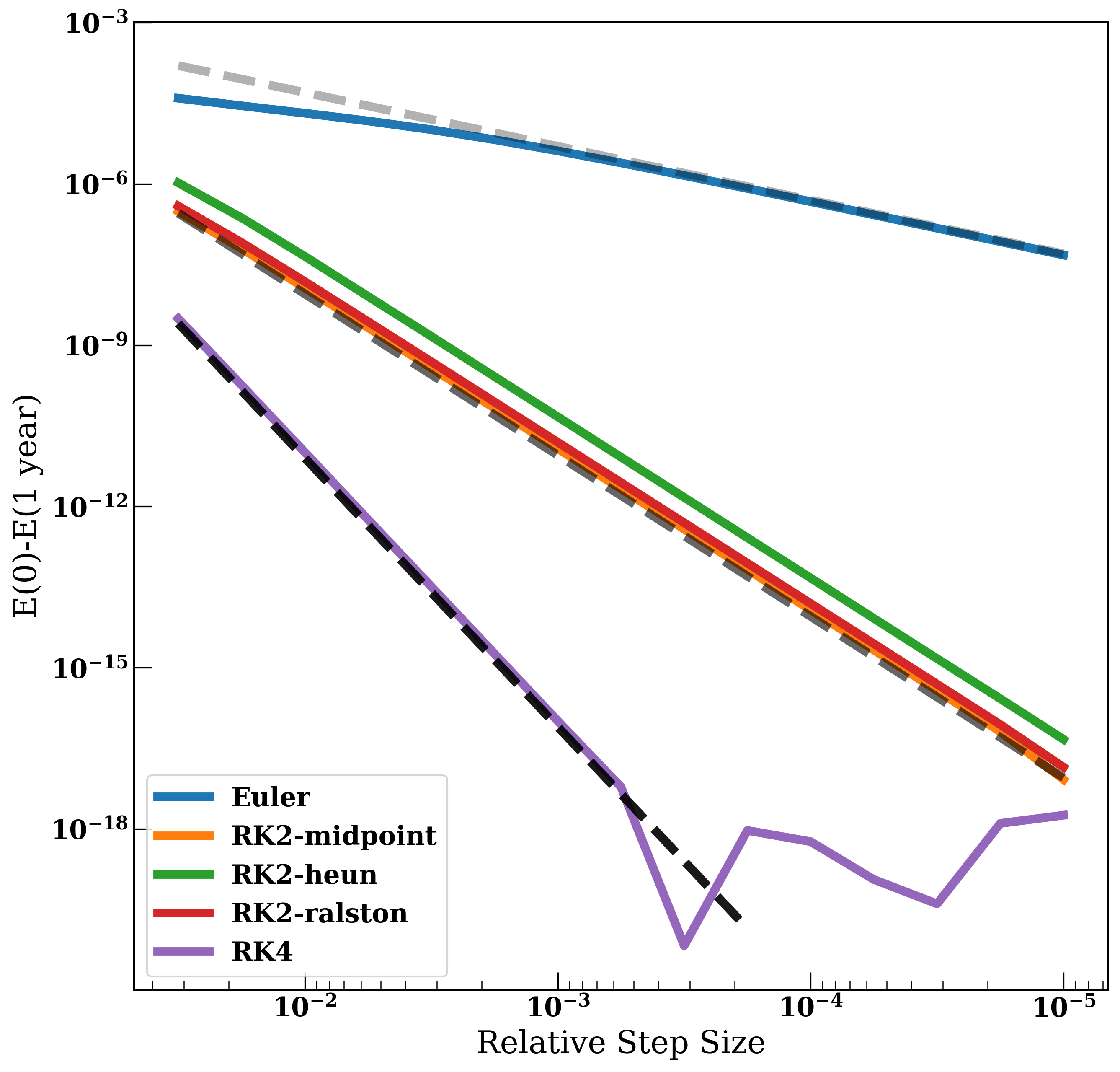
The energy error over an orbit of each of our methods as a function of timestep. The lines have slopes \( (\Delta t)^{1} \), \( (\Delta t)^{3} \), \( (\Delta t)^{5} \)
Here we see that, for sufficiently small step size, the Euler method's error decreases linearly with the timestep, the second order methods decrease with the third power of timestep, and the fourth order with the fifth order of the timestep. It's also worth noting the difference in error between integrators of the same order, but different coefficients are much smaller than the difference between orders. It's for this reason that the specific integration method is often not specified precisely in most applications - in favor of simply referring to the order of the integrator. Finally, it's worth noting that these increases in accuracy cannot occur forever. Eventually, for a small enough timestep, machine precision limits are reached, and the accuracy evolves in a more stochastic fashion. We can see that this occurs rapidly for our fourth-order integrator.
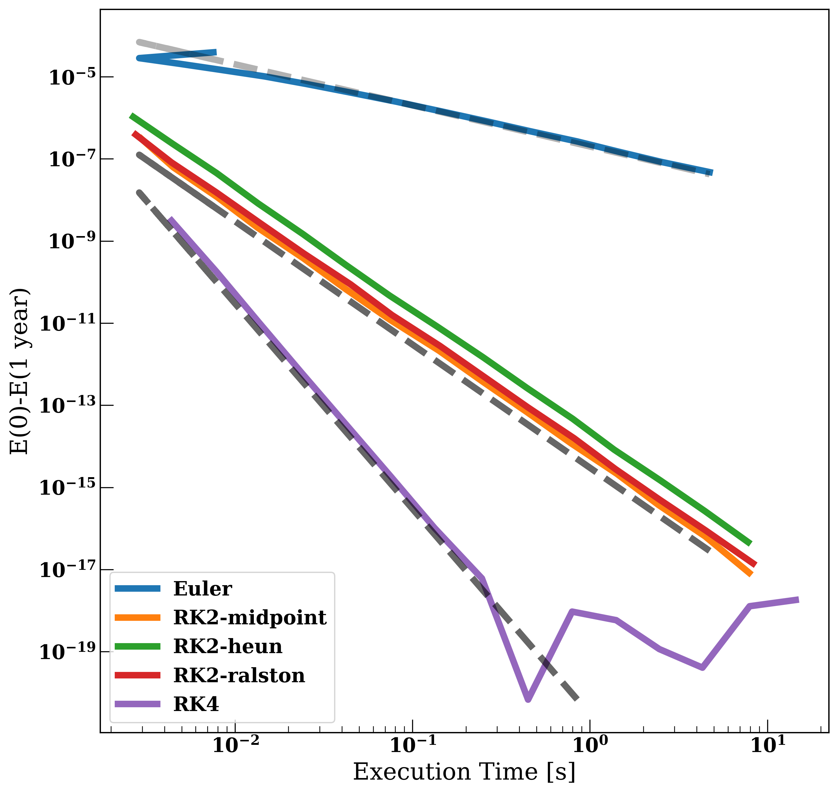
Finally, there's the question of efficiency. Even if the accuracy of a high-order integrator is better at small timesteps, high-order integrators are also more numerically complicated than low-order integrators and hence run slower. It's then worth asking, for a given level of accuracy, do high-order integrators with large timesteps, solve the equations of motion faster than those of low-order and small timesteps? We can test this by showing the energy error of our integrators vs the execution time.
The energy error over an orbit of each of our methods as a function of execution time. The lines have slopes \( (\Delta t)^{1} \), \( (\Delta t)^{3} \), \( (\Delta t)^{5} \)
This shows that in general, the greater overhead from a high order integrator is more than compensated by it's increased accuracy. Hence, in general, if one wishes to solve a problem with high accuracy as quickly as possible high order integrators are the best choice. Note that if only very low accuracy is required the differences between the integrator of different orders become smaller - but there are few applications for which numerical integrators at low accuracy are required, so in practice this approach is rare.
Multistep Methods
Runge-Kutta methods require a large number of computations for each step, as - especially for higher order integrators the \(k\)s must be recomputed at every step. An alternative to this is multistep methods, which compute the next step as a linear function of previous steps. One of the most commonly used types of multistep methods is linear multistep, of which the Adams-Bashforth methods are most well known. The central insight that leads to the Adams-Bashforth method is writing the step as the integral of the function's derivative. So for \(\frac{dy}{dt} = f(t,y(t)) \).
$$ y(t+ \Delta t) = y(t) + \int_{t} ^{t+\Delta t} f(t) dt$$
the integral is then interpolated using lagrange polynomials. If the polynomial interpolant points are taken to be equally spaced, in the case of a third order scheme:
$$(x_0 = t, y_0 = f(t))$$
$$(x_1 = t+ \Delta t),y_1 = f(t + \Delta t))$$
$$(x_2 = t+ 2 \Delta t),y_2 = f(t + 2\Delta t)$$
the interpolating polynomial can then be computed from these points. With the basis functions given by
$$b_j(x) = \prod_{0 \leq m \leq k, m \neq j} \frac{x-x_m}{x_j -x_m}$$
with the interpolation given by
$$L(x) = \sum_{j=0}^k y_j b_j(x)$$
For our example the polynomial takes the form
$$f(t,y(t)) \approx \frac{(-\text{$\Delta $t}+t-\tau ) (f(t) (-2 \text{$\Delta $t}+t-\tau
)+(t-\tau ) f(t-2 \text{$\Delta $t}))-2 (t-\tau ) f(t-\text{$\Delta $t})
(-2 \text{$\Delta $t}+t-\tau )}{2 \text{$\Delta $t}^2}$$
This interpolation can be used as an approximate functional form for f. While complicated, such an object is just a polynomial and is thus easy to integrate and, since it is a simple polynomial in \( x \) it can be integrated. It's convenient to take \( \tau \rightarrow t + u \Delta t \). This transforms our integral to
$$ y(t+ \Delta t) = y(t) + \int_{0} ^{1} \ f(u) \Delta t du$$
in our case the result is
$$ y(t+ \Delta t) \approx y(t) + \frac{23}{12} \text{$\Delta $t} f(t)+\frac{5}{12} \text{$\Delta $t} f(t-2
\text{$\Delta $t})-\frac{4}{3} \text{$\Delta $t} f(t-\text{$\Delta $t})$$
Hence, we obtain a recursive scheme as a function of the previous steps. It's important to note that the Adams-Bashfoth methods are not self-starting, so given an initial condition \( t_0 \), the first few steps have to be computed with some other method. However, after these steps are computed, Adams Bashforth methods often are faster than Runge-Kutta due to the decreased computational load, as previous steps can be stored and used to compute subsequent steps.
An integration of the earth's orbit using the second-order Adams-Bashforth Method.
An integration of the earth's orbit using the third order Adams-Bashforth Method.
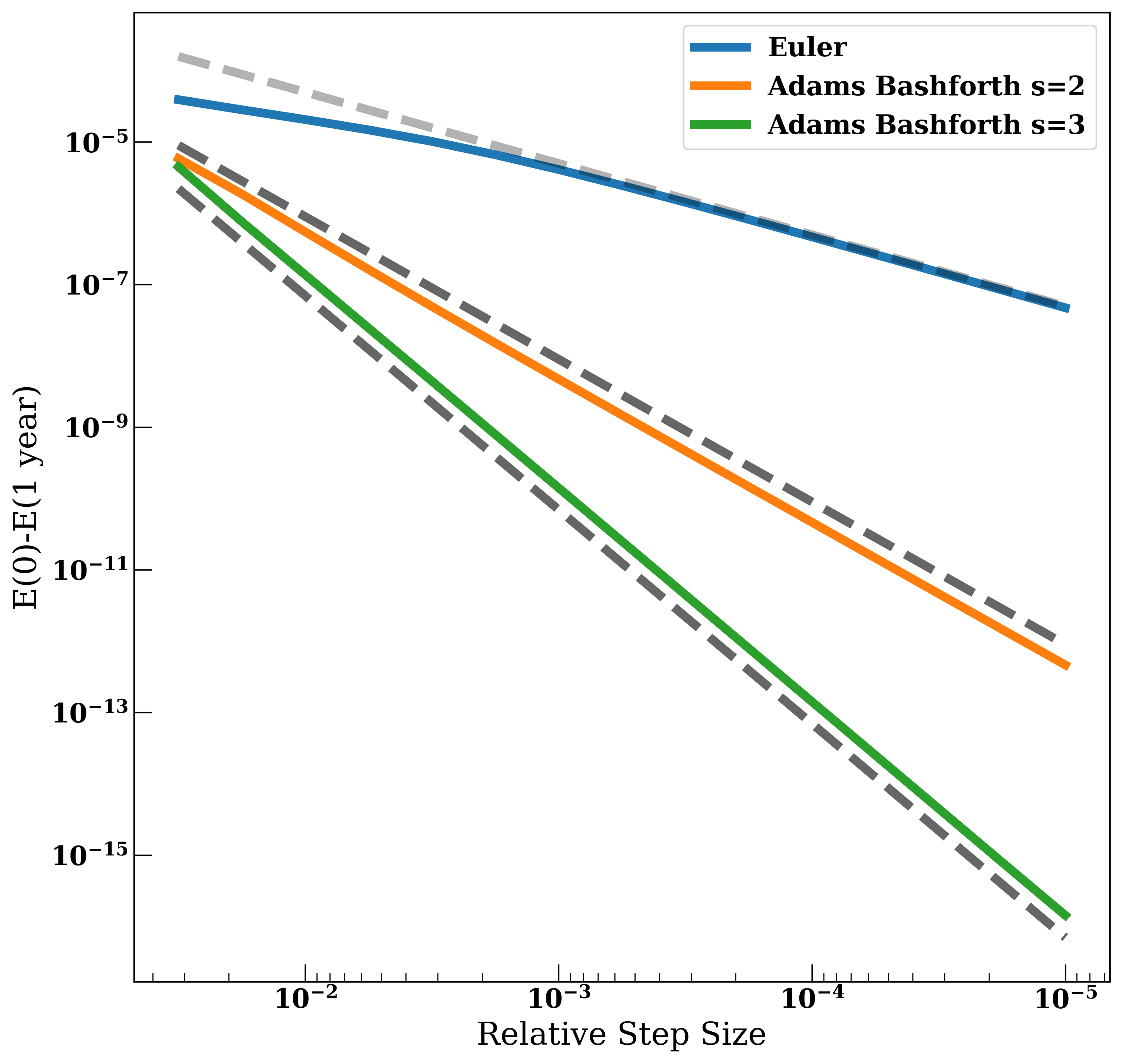
Finally we can confirm that the behavior behaves as we expect with stepsize.
The energy error over an orbit of each of our methods as a function of execution time. The lines have slopes \( (\Delta t)^{1} \), \( (\Delta t)^{2} \), \( (\Delta t)^{3} \)
Equation Stiffness
Stiffness is a property of some systems of differential equations where some numerical methods to approximate the solution become numerically unstable for reasonable step sizes. These instabilities can take many forms and can take the form of wild oscillations or failure to converge to the true solution until the step size becomes very small. Interestingly, an exact definition of stiffness is difficult to come by, hence it's often best to examine the solutions given by numerical schemes to try and detect problematic behavior. That said, a good rule of thumb is that differential equations are often stiff if they contain widely varying timescales (e.g a short period of significant decay or growth), if explicit methods work only extremely slowly, of if the eigenvalues of the Jacobian of the system differ greatly in magnitude.
The traditional example of a stiff system is the following problem
$$ \frac{dy(t)}{dt} = -15 y(t) $$
this differential equation is linear and thus has a closed form solution \( y(t) = e^{15 t} \). This exponential behavior is our first clue that this equation may be stiff. We can confirm our solution by solving the equation using the forward Euler method.
The convergence of the Euler method on a stiff system
Note that the solution oscillates widely about the true solution for large step sizes, and only converges when the step size becomes extremely small. We can take a closer look at the projected solutions for a given timestep by plotting only those
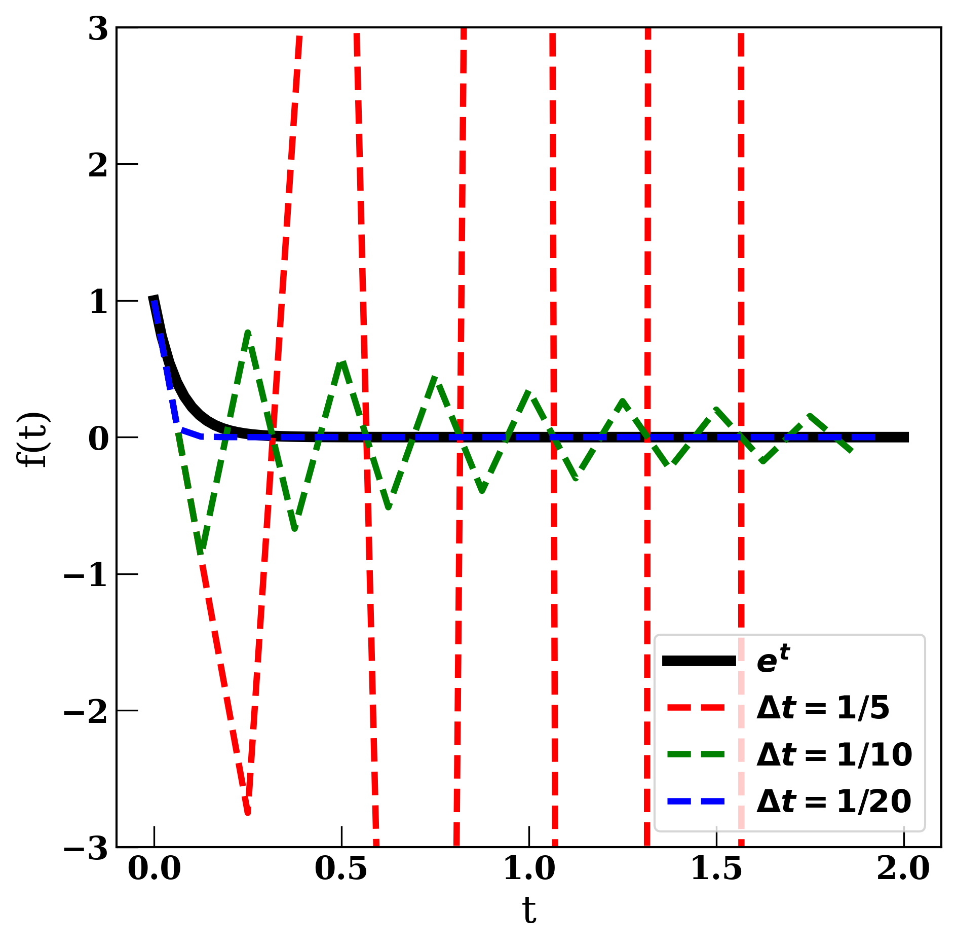
Euler method convergence on the same system for \( (\Delta t) = 1/5, 1/10 \) and \(1/20 \)
We can clearly see three different types of behavior. For very small timesteps \( \Delta t = 1/5 \) our approximation to the solution oscillates widely about the true solution with increasing amplitude as \( t \rightarrow \infty \). For smaller timesteps \( \Delta t = 1/10 \) we recover the correct behavior in the \( t \rightarrow \infty \) limit, however, there are still large oscillations that are not present in the true solution. Finally, for the smallest timesteps \( \Delta t = 1/20 \) we see no oscillations, but there is a bias at small \(t \), where the numerical solution is significantly smaller than the true solution.
These oscillations are caused by the Euler integration method losing its stability for larger timesteps. In general, this sort of behavior can arise in any integrator, though the Euler method in particular is often unstable. The Runge-Kutta method tends to exhibit better stability properties whereas the Adams-Bashforth is prone to instability. This weakness means Adams-Bashforth methods, particularly those of higher orders aren't used as often as Runge-Kutta methods.
Now that we've described a case of stiffness we turn our focus back to celestial mechanics. In this case, the source of stiff-like behavior is often sharply changing interaction timescales, typically caused by the velocities of particles changing suddenly. This occurs most often in the case of close encounters between bodies, or for single bodies on highly eccentric orbits. To demonstrate this we can integrate the orbit of a comet using the midpoint method. This comet has an orbital period of many years, hence we'll take our timesteps to be relatively large \( \Delta t = 0.01 \) years and \( \Delta t = 0.05 \) years. Since these are much shorter than the comet's orbital period we expect to both simulations will be well converged and exhibit little error.
Orbits and energy over time for the integration of a comet's orbit at two different timesteps.
Despite expectations we see that the larger timestep has huge spikes in its energy error that correspond to its periapsis passage. These spikes result in visible precession of the orbit - which should not occur in an unperturbed two-body system. Similarly, our smaller timestep exhibits similar but less obvious behavior. In both, this behavior is a consequence of the comet's increased velocity near periapsis. The high-velocity results in fewer steps being taken per unit of distance traveled and effectively undersampling during part of the orbit.
Impicit Methods
Having seen ways that system stiffness can stymie numerical integration. We now introduce implicit integration methods, which often have better stability properties than their explicit counterparts. Implicit methods differ from their explicit counterparts, in that for implicit methods, the next step \( y(t + \Delta t) \) must be written in terms of itself, not just previous terms. The simplest example of such a method is the backward Euler method. Here
$$y(t+\Delta t) \approx y(t) + \Delta t f(t+\Delta t, y(t+\Delta t))$$
If we apply this scheme to our stiff equation, we end up with the following condition:
$$ \frac{y(t)-y(t+\Delta t)}{\Delta t} = - 15 y(t + \Delta t)$$
in the case of such a simple equation, this can be solved explicitly for \( \Delta t \). It's straightforward to show that this condition is equivalent to
$$ y(t+\Delta t) = \frac{y(t)}{1 + 15 \Delta t} $$
We can see the results of applying the iteration below.
The convergence of the Euler method on a stiff system
There are two things worth noticing in comparison to the explicit Euler method. First is the lack of oscillations even for relatively large timesteps. This is a general property of implicit methods - they often have far more desirable stability properties than their explicit counterparts. The second is that the implicit Euler method approximates our true function from the top - rather than from the bottom. This inverted behavior of the error is typical for implicit methods. We can see this by applying this same logic to a n-body problem, however, in the case of the n-body problem, no closed form exists for the next step in terms of the previous step. Hence, solving for \( y(t+\Delta t) \) must be done numerically.
One way to do this is to compute a trial \( y_0'(t+\Delta t) \) through
$$y_{n+1}'(t+\Delta t) = y(t) + \Delta t*f(y_{n}'(t+\Delta t) )$$
We can iterate this process over and over, each time checking the difference \( y_{n+1}'(t+\Delta t) - y_{n}'(t+\Delta t) \) is smaller than some threshold. After a few iterations (typically \(n \approx 3-4 \)) we will find that \( y_{n+1}'(t+\Delta t) \) converges to \( y(t+\Delta t) \). If we implement this for the Euler method, we obtain the following result:
Integrating the orbit of earth with the implicit Euler method.
As expected of an implicit method, the energy behaves opposite to that in the explicit Euler, and the planet rapidly spirals into the star. It's worth noting that we've done an awful amount of work simply to implement a first-order method, and at each step, an iterative process is needed to solve our equations. All of these processes are slow. Hence, while implicit integrators tend to have better stability properties they're not used often in scientific applications, due to speed concerns. However, they remain a great choice for integrating stiff systems of many kinds. Many of the integration methods we've discussed thus far have implicit analogies, they include implicit Runge-Kutta methods and the Adamas-Moulton methods (an implicit variant of Adams-Bashforth)
Predictor Corrector Methods
Predictor-Corrector methods typically combine explicit and implicit methods. They consist of a two-step process, first one method - typically an explicit method is used to generate a guess of the next timestep based on the previous timesteps, we'll call this \( y'(t+\Delta t) \).
Then in a second step, typically using an implicit method, using our approximate next timestep \(y'(t+\Delta t) \) is used to refine a prediction for \( y(t+ \Delta t) \). The simplest predictor-corrector combines the explicit forward Euler method with the implicit Adams-Moulton method of order 2, also known as the trapezoidal rule. these methods are described by the following iterations:
$$y(t+\Delta t) = y(t) + \Delta t f(t, y(t))$$
$$y(t+\Delta t) = y(t) + \frac{\Delta t}{2} \left( f(t, y(t)) + f(t+\Delta t, y(t+\Delta t)) \right)$$
since the predictor corrector scheme uses the output of the explicit method as the input to the implicit one, the following iteration results:
$$y'(t+\Delta t) = y(t) + \Delta t f(t, y(t))$$
$$y(t+\Delta t) = y(t) + \frac{\Delta t}{2} \left( f(t, y(t)) + f(t+\Delta t, y'(t+\Delta t)) \right)$$
We can see an example of this method applied to the Earth-Sun system below.
Integrating the orbit of earth with the Euler method corrected with the trapezoidal method.
It performs much better than the standard Euler method, without much extra computational cost. It's also worth noting that since the Euler method is simply a first-order Adams-Bashforth method. Hence, we've combined an Adams-Bashforth method with an Adams-Moulton method of different orders. This works generally, and often predictor-corrector schemes can be extended to higher orders by using a combination of the Adams-Bashforth and Adams-Moulton schemes. They typically have stability properties in between those of explicit methods and those of implicit methods.
Adaptive Integrators
When working with n-body problems, the most common source of stiffness comes from close encounters between two bodies, either due to scattering events or eccentric orbits. It is therefore desirable to have an integrator that is resistant to such velocity changes. One approach to doing this is to vary the timestep of the integrator, shrinking it during these close approaches. This approach might be slightly slower than simply using a constant timestep, but it ensures the result remains precise. Here we construct the Dromand-Prince adaptive method - a special case of the Runge-Kutta methods - which serves as the default in several popular integration packages including Matlab, Octave, and SciPy. In Dormand-Prince we start by computing the following seven \( k_i \).
$$k_1 = \Delta t f(t,y(t))$$
$$k_2 = \Delta t f(t+\frac{1}{5}\Delta t ,y(t + \frac{k_1}{5}))$$
$$k_3 = \Delta t f(t+\frac{3}{10}\Delta t ,y(t + \frac{3 k_1}{40} + \frac{9 k_2}{40} ))$$
$$k_4 = \Delta t f(t+\frac{4}{5}\Delta t ,y(t+ \frac{44 k_1}{45} - \frac{56 k_2}{40} + \frac{32 k_3}{9} ))$$
$$k_5 = \Delta t f(t+\frac{4}{5}\Delta t,y(t + \frac{19372 k_1}{6561} - \frac{25360 k_2}{2187} + \frac{64448 k_3}{6561} - \frac{212 k_4}{729} ))$$
$$k_6 = \Delta t f(t+\Delta t,y(t + \frac{9017 k_1}{3168} - \frac{355 k_2}{33} - \frac{46732 k_3}{5247} \frac{49 k_4}{176} - \frac{5103 k_5}{18656} ))$$
$$k_7 = \Delta t f(t+\Delta t,y(t + \frac{35 k_1}{384} - \frac{500 k_3}{1113} + \frac{125 k_4}{192} - \frac{2187 k_5}{6784} - \frac{11 k_6}{84} ))$$
Finally we can compute the next timestep to fourth order using the typical Runge-Kutta expansions, we'll call this result \(y'(t+\Delta t) \)
$$y'(t + \Delta t) = y(t) + \frac{35 k_1}{384} - \frac{500 k_3}{1113} + \frac{125 k_4}{192} - \frac{2187 k_5}{6784} - \frac{11 k_6}{84}$$
the next part of the Dorman-Prince alogrithm involves additionally computing the value of the next step at fifth order, which we'll call \(y'(t+\Delta t) \)
$$y(t + \Delta t) = y(t) + \frac{35 k_1}{384} - \frac{500 k_3}{1113} + \frac{125 k_4}{192} - \frac{2187 k_5}{6784} - \frac{11 k_6}{84}$$
Note that in order to do both of these calculations, we only had to compute the \(k_i\) once, then we could reuse them to produce both 4th and 5th order methods. Further, we can now use the difference between these values \( | y'(t + \Delta t) - y(t + \Delta t)| \) as an estimate of the error. We expect our integrator to have errors of order \( C (\Delta t)^5 \). Hence we can update our timestep by
$$(\Delta t)_{new} = \left(\frac{\tau}{ | y'(t + \Delta t) - y(t + \Delta t)|} \right)^{1/5} (\Delta t)_{old}$$
The result of this work applied to the comet system is shown below, for \( \tau = 10^{-12}\) .
Integrating the orbit of a comet with the Dormad-Prince method.
Here we show the state of the orbit, the timestep, and the energy error as a function of time. We can see that at periapsis the timestep drops, allowing for greater resolution when the system changes rapidly. This effect is visible in the orbit animation, which slows down near periapse and runs more quickly when the comet is far from the star. This results in an energy error that slowly drifts over time, this behavior is much more like our Runge-Kutta integrations of circular orbits and exhibits no jumping near periapse.
Sympletic Integrators
Thus far, we've examined several different types of integrators and how they respond to different conditions found in celestial mechanics. All the integrators we've shown have energies that drift over time, and while this drift can be mitigated - say by using adaptive integration methods - we've yet to see it be eliminated completely.
fortunately, such integrators exist. The simplest example of such an integrator is the leapfrog method. In these cases, the positions and velocities are updated in different ways, with a given step being broken down into substeps. For example, if the leapfrog method is applied to a celestial mechanics problem with positions \( r_i \) , velocities \(v_i \), and accelerations \(a_i(r_i) \)
$$v_i(t + \frac{\Delta t}{2}) = v_i(t) + a_i(r_i(t)) \frac{\Delta t}{2}$$
$$r_i(t + \Delta t) = r_i(t) + v_i(t + \frac{\Delta t}{2}) \Delta t$$
$$v_i(t + \Delta t) = v_i(t) + a_i(r_i(t+\Delta t)) \frac{\Delta t}{2}$$
This method 'kicks' the velocity for half a timestep using the instantaneous acceleration, then lets the positions 'drift' according to that new velocity for a full timestep, before once again 'kicking' the velocity with the interpolated acceleration term. For this reason, the leapfrog integrator is sometimes referred to as a 'kick-drift-kick' method. If we implement the leapfrog integrator on an orbital problem, we get the following behavior.
Integrating the orbit of the earth with Leaprfog method.
This method has very different behavior from our Runge-Kutta schemes, rather than linearly increasing or decreasing - the energy instead oscillates about a single value. This is highly desirable for simulating systems of planets, especially over many orbits where the drift in energy may start to matter.
As with the Runge-Kutta integrators, there are also higher-order versions of symplectic integrators. In general, the algorithms split the integration of a single step into j substeps. With
$$r_{i+1} = r_i + c_i v_{i+1} \Delta t$$
$$v_{i+1} = v_i + d_i a_{i+1}(r_i) \Delta t$$
Higher order integrators can then be constructed by specifying the coefficients \( c_i \) and \( d_i \). Below we implement the third and fourth-order integrators found by Ronald Ruth and apply to use them to integrate the orbit of Earth. The coefficients are:
$$ c_1 = 1, c_2 = -2/3, c_3 = 2/3, d_1 = -1/24, d_2 = 3/4, d_3 = 7/24 $$
for the third order integrator, and
$$ c_1 = c_4 = \frac{1}{2(2-2^{1/3}}, c_2 =c_3 = \frac{1-2^{1/3}}{2(2-2^{1/3}}, d_1 = d_3 = \frac{1}{2-2^{1/3}}, d_2 = -\frac{2^{1/3}}{2-2^{1/3}}, d_4 = 0 $$
for the fourth order integrator.
Integrating the orbit of the earth with the third order Ruth Integrator.
Integrating the orbit of the earth with the fourth order Ruth Integrator.
We can see that as we go to higher order, the size of the oscillations decreases - but they stay bounded over the course of the integration.
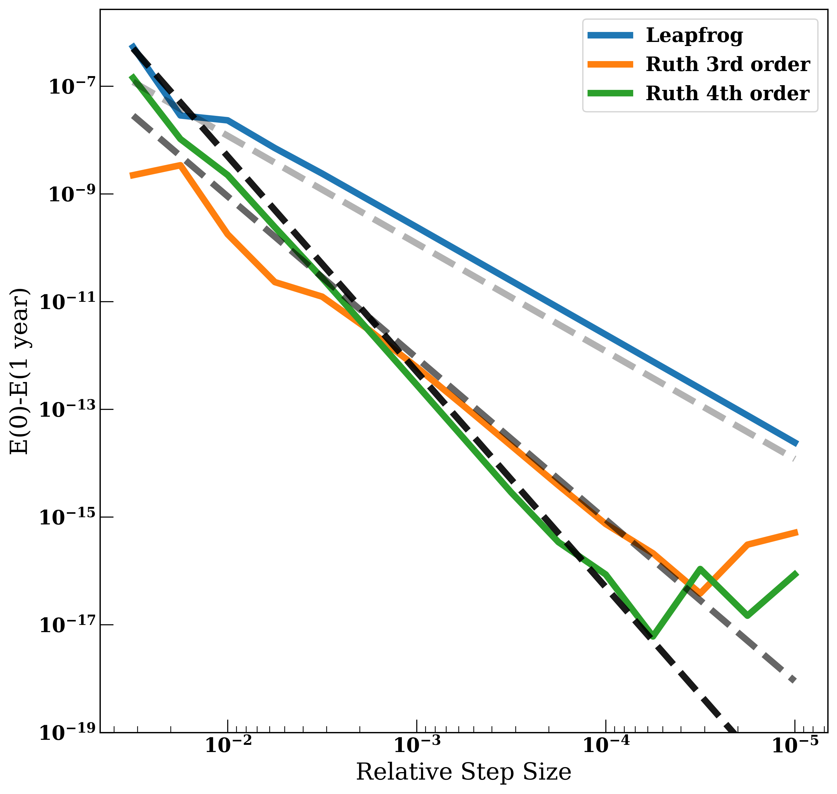
Finally, we can verify that our integrators do indeed have the convergence properties we claim, by testing their energy errors over an orbit as a function of the timestep.
The energy error over an orbit of each of our methods as a function of execution time. The lines have slopes \( (\Delta t)^{2} \), \( (\Delta t)^{3} \), \( (\Delta t)^{4} \)