The Two Body Problem

The solution to the two-body problem forms the foundation of much of celestial mechanics. Hence, while simple, any discussion of celestial mechanics without treatment of the two-body problem would be incomplete. The basic setup is to consider the motion of two point masses \(m_1\) and \(m_2\) acting under mutual gravitational attraction with the force \[ \vec{F_{12}} = m_1 \frac{d^2 \vec{r_1}}{dt^2} \] \[ \vec{F_{21}} = m_2 \frac{d^2 \vec{r_2}}{dt^2} \] according to Newton's second law. \(F_{12} = -F_{21}\). Now we can consider the center of mass of the system, located at \[ \vec{r}_{cm} = \frac{m_1 \vec{r_1} + m_2 \vec{r_2}}{m_1+m_2} \] Let's find the acceleration of this point, since \[ \frac{d^2 \vec{r}_{cm}}{dt^2} = \frac{1}{m_1+m_2} \left(m_1 \frac{d^2 \vec{r_1}}{dt^2} + m_2 \frac{d^2 \vec{r_2}}{dt^2} \right) \] In other terms, \[ \frac{d^2 \vec{r}_{cm}}{dt^2} = \frac{1}{m_1+m_2} \left(\vec{F_{12}} + \vec{F_{21}} \right) = 0 \] If the acceleration is zero, the center of mass moves with a uniform, constant velocity in some direction. Now we consider the difference of these two vectors, \(\vec{\delta r} = \vec{r_1} - \vec{r_2\). We can also find the acceleration of this difference as \[ \frac{d^2 \vec{\delta r }}{dt^2} = \frac{\vec{F_{12}}}{m_1} - \frac{\vec{F_{21}}}{m_2} \] Since the forces are equal and opposite, this reduces to \[ \mu \frac{d^2 \vec{\delta r }}{dt^2} = \vec{F_{12}} \] Where \( \mu = \frac{m_1 m_2}{m_1+m_2} \) is the reduced mass. This is the same form as the one-body problem. Finally, we note that our original vectors can be written in terms of \( \vec{r}_{cm} \) and \( \vec{\delta r} \). \[ \vec{r_1} = \vec{r}_{cm} + \frac{m_2}{m_1+m_2} \vec{\delta r} \] \[ \vec{r_2} = \vec{r}_{cm} + \frac{m_1}{m_1+m_2} \vec{\delta r} \] Since the motion \( \vec{r}_{cm} \) is trivial, as the center of mass moves in a straight line, all of the interesting physics comes from that of \( \vec{\delta r} \), which is just a one-body problem. Hence, when in the center of the mass frame, the two-body problem is equivalent to just two scaled one-body problems - with each mass tracing out its solution independently of the other.

The One-Body Problem

Now the only thing we have left to solve is the one-body problem. \[ m \frac{d^2 \vec{\delta r }}{dt^2} = \vec{F_{12}} \] Since two-body motion is planar, we can now solve this equation in polar coordinates. \[ m \left\{ \frac{d^2r}{dt^2} - r \left(\frac{d\theta}{dt}\right)^2, r \frac{d^2\theta}{dt^2} + 2 \frac{dr}{dt} \frac{d\theta}{dt} \right\} = \left\{ -\frac{G M m}{r} , 0 \right\} \] Since there's no acceleration in the \( \theta \) direction, angular momentum is constant, \( L = m r^2 \frac{d\theta}{dt} \). Thus, the problem reduces to a single radial equation: \[ \frac{d^2r}{dt^2} - r \left(\frac{d\theta}{dt}\right)^2 = -\frac{G M}{r} \] This can be written in terms of angular momentum as \[ \frac{d^2r}{dt^2} = -\frac{G M}{r} + \frac{L^2}{m^2 r^3} \] This equation is still tough to solve. Two tricks and final steps are necessary to make it tractable. The first is to rephrase it in terms of \( u = 1/r \). The second is to notice that our expression for angular momentum implies \[ dt = \frac{L u^2}{m} d\theta \] Hence \[ \frac{dr}{dt} = \frac{d}{dt} \frac{1}{u} = -\frac{1}{u^2} \frac{du}{dt} = - \frac{L}{m} \frac{du}{d\theta} \] Finally, we can transform our equation into \[ \frac{d^2u}{d\theta^2} + u = \frac{G M m^2}{L^2} \] This equation has a known solution! Transforming back to \( r \) we have \[ \frac{1}{r} = \frac{G M m^2}{L^2} + k \cos(\theta) \] for some constant \( k \). This is exactly the equation of an ellipse, with the source of attraction at one focus.

As always, seeing is believing. Here we show the solution to the two-body problem for the circular case for varying different mass ratios. In every case, the motion is equivalent to two one-body problems moving about a common center of mass. In addition, the logo of this site also exhibits two-body motion, but in the eccentric case. We can see in that case the motion is still equivalent to one-body motion about the center of mass!

Kepler elements

Thus far we've found that Kepler orbits are ellipses. These ellipses are often described in terms of 6 main Kepler elements. They are:

Semi-major axis (a). This element parameterizes the size of the ellipse along its longest diameter. Alternatively, it's the length of the line segment that runs through both foci of the ellipse. An orbit can theoretically have any semi-major axis, but very large semi-major axes are only weakly bound to their hosts, and very small semi-major axes may impact their hosts.

Eccentricity (e). The eccentricity is a value from \(0 \leq e \leq 1 \) and parameterizes the shape of the ellipse. For \( e =0 \) the resulting ellipse is a circle and as \( e \) increases the ellipse becomes more stretched out, eventually becoming parabolic for \(e=1 \).

True Anomaly (\(\nu\) or \(\theta\) or \(f\) ). The true anomaly parameterizes the location of a body in its orbit. It is the angle between the body's periapsis and its current position as seen from the focus point of the ellipse. As an angle \(0 \leq \nu \leq 2\pi \)

With these three elements, we've managed to specify the shape and size of an orbit and the position of a body in that orbit. What's left is to specify the orientation of the orbit with respect to some reference frame. The classic approach to this is to do so by specifying three angles. Orienting an object in 3D space is a general problem and different solutions include rotation matrices, Euler angles, or some other type. In our case, the traditional three angles are the inclination, argument of periapsis, and longitude of the ascending node.

Inclination (i). The inclination parameterizes the tilt of the ellipse relative to some reference plane. As an angle, it can take any value from \(0 \leq i \leq 2\pi \), with values greater than \( \pi/2 \) and less than \( 3\pi/2 \) describing retrograde motion.

Argument of periapsis ( \( \omega \) ). The argument of periapsis parameterizes the orientation of the ellipse with respect to the orbital plane. In other words, it sets the angle of periapse passage with respect to some reference plane, as an angle \(0 \leq \omega \leq 2\pi \).

Lnongitude of the Ascending Node ( \( \Omega \) ). The longitude of the ascending node parameterizes the orientation of the ascending node of the ellipse with respect to some reference plane. Any ellipse will pass through a plane intersecting its center at two points. The ascending node is the point where the orbit passes from the negative to positive coordinates in the reference plane. Like \( \omega \), \( \Omega \) can take any value \(0 \leq \Omega \leq 2\pi \). We can play with these coordinates in the graphic below to help get an understanding of the role of each.

There are also several derived elements that bear mentioning. These elements are functions of the 6 basic Kepler elements and are often mathematically useful. The most common ones are:

Mean anomaly ( \( M\)). Like the true anomaly, the mean anomaly parameterizes the position of a planet in its orbit. However, the mean anomaly is linearly related to time, with \( M = n(t-t_0) \) with \( n = \frac{2 \pi}{P} \) where \( P \) is the body's orbital period. While convenient mathematically, it does not, in general, correspond to any physical angle in an orbit.

Eccentric anomaly ( \(E \)). Like the true anomaly, the eccentric anomaly parameterizes the position of a planet in its orbit. It can be related to the true anomaly by \( \tan(\nu/2) = \sqrt{\frac{1+e}{1-e}}\tan(E/2) \)

Hamiltonians

Up until now we've stuck to the Newtonian version of classical mechanics. In general the Newtonian approach adopts the following strategy for solving a nbody problem.

1. Write out all the forces
2. Use F=ma to derive a system of differential equations governing the bodies' behavior (these are the equations of motion).

There's nothing physically incorrect about this approach, at least in classical mechanics it will always result in the correct equations of motion - if done correctly. However, this caveat is a significant one. Consider writing out the differential equations governing the general three-body problem. First, since each body lives in a three-dimensional space, F will be a vector with three components. Each of the three bodies will then have its own equations of motion, which will be a function of the positions of the other bodies. This results in a total of 9 scalar coupled differential equations to be numerically solved. This is certainly a challenge!
The Hamiltonian formalism changes things by defining the Hamiltonian of a system H as the sum of its kinetic and potential energies \( H = T+V \). The exciting thing about this formalism is that the equations of motion can be written simply using Hamilton's equations, i.e. $$\frac{d\vec{q}}{dt} = \frac{\partial H}{\partial \vec{p}}$$ and $$\frac{d\vec{p}}{dt} = -\frac{\partial H}{\partial \vec{q}} $$ Where here \( \vec{q} \) and \( \vec{p} \) are the canonical positions and canonical momenta of the system. The advantage of this method is that all the dynamics of a system can be encoded into a single object - the Hamiltonian - upon which all the equations of motion depend. Not all systems can be written in this way, but in general, systems that conserve energy can. Hence, analysis of the Hamiltonian itself is often sufficient to reach conclusions about the system. However, this formulation immediately raises an important question. What makes these coordinates 'canonical'

Canonical Coordinates

For a set of coordinates to be canonical three conditions must be met. $$\{q^i,q^j\} = 0$$ $$\{p_i,p_j\} = 0$$ $$\{q^i,p_j\} = 0$$ where here we've written our condition in terms of the Poisson bracket. The Poisson bracket is defined as follows: $$\{f,g\} = \sum_{i=1}^N ( \frac{\partial f}{\partial q_i} \frac{\partial g}{\partial p_i} - \frac{\partial f}{\partial p_i} \frac{\partial g}{\partial q_i})$$

Pendulum Example

While our main goal is to understand celestial mechanics; it's worth testing our knowledge on simpler systems first. Consider the case of the motion of a pendulum. Its motion can be characterized by some angle \theta with potential energy written as \( V(\theta) = m g l (1- cos(\theta)) \) and its kinetic energy \( \frac{1}{2} m l^2 (\frac{d\theta}{dt})^2 \). The Lagrangian is therefore: $$L = \frac{1}{2} m l^2 (\frac{d\theta}{dt})^2 - m g l (1- cos(\theta)) $$ We've parameterized the motion with position \( \theta \) but we need the conjugate canonical momentum. 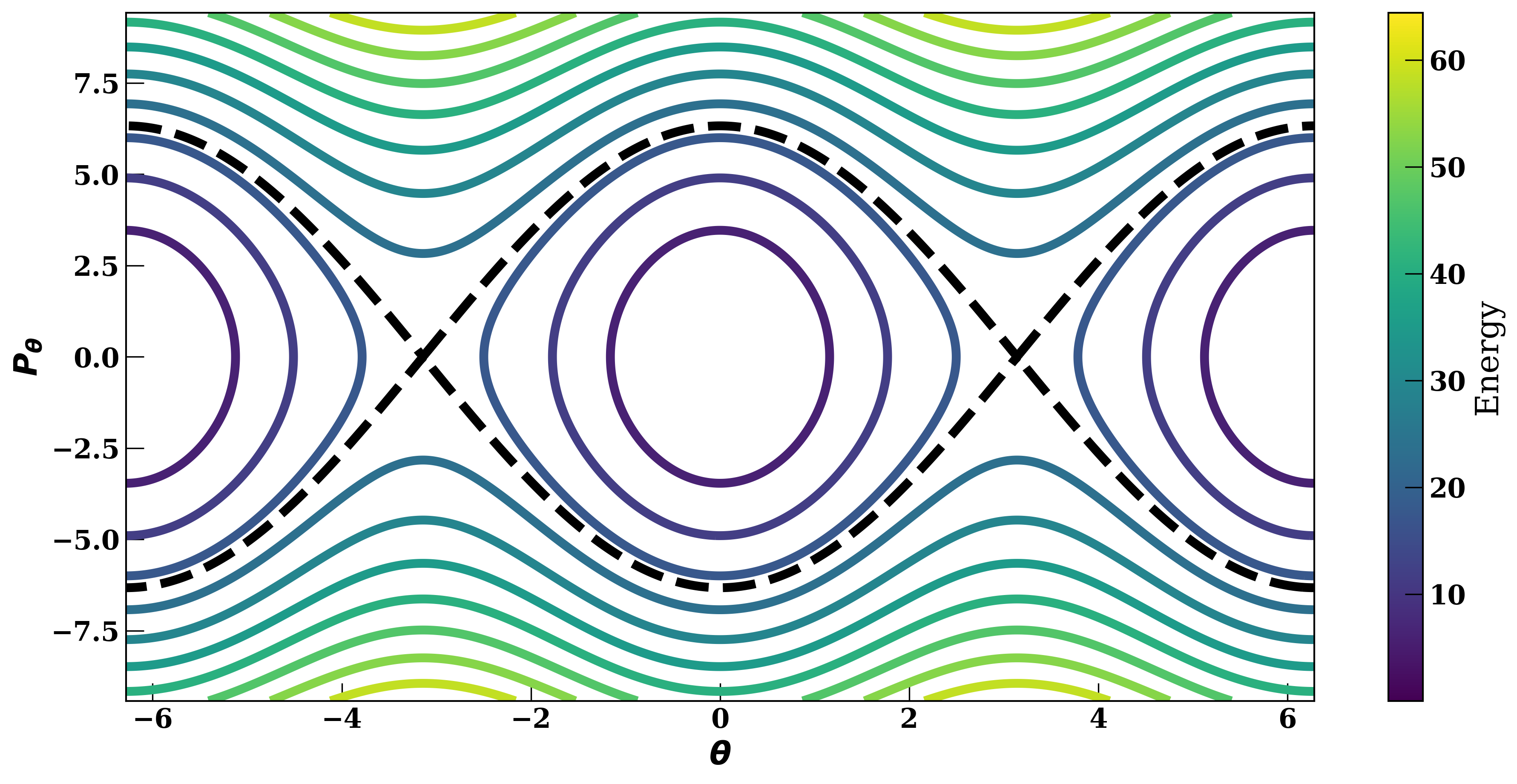To find this we appeal to $$P_{\theta} = \frac{\partial L}{\partial \dot\theta} = m l^2 \dot\theta$$ It's Hamiltonian is then - in terms of conjugate coordinates $$H = \frac{P_\theta^2}{2 m l^2} + m g l (1 - \cos(\theta)) $$ Finally, since our Hamiltonian is a function of two dynamical variables \( (P_\theta, \theta) \) we can now plot the energies of the pendulum as a function of those constants. The result is the following plot.

Ths plot tells us a lot about our system.

1. Since energy is conserved along our contours, the only freedom our system has to move - from a given set of initial conditions - is along those contours. Hence, these contours also correspond to the trajectories through Hamiltonian Phase Space.

2. There's a clear separation between two different types of trajectories here (shown by our dashed black line). Inside the black line trajectories curve back on themselves and explore only a small range of \( \theta \). Outside the line, they loop across the entire domain. This black line is referred to as a separatrix and separates topologically distinct regions of the phase space. In this case, we have a bit of intuition about the problem and can physically interpret these different states. The closed curves result in an oscillation about zero and occur when the momentum is low. This corresponds to approximately harmonic oscillation about \( \theta = 0 \). The open curves explore all theta and occur when momentum is large - this must correspond to the case where the pendulum is swinging fully around its pivot point.
Overall, hamiltonian phase space gives us tools to gain significant insight into physical systems - however, it comes at the cost of pushing those systems into large numbers of dimensions. In our 1D case, we have a two-dimensional Hamiltonian phase space; more generally for \(N\) differential equations, we can expect phase space to be \(2N\) dimensional. This also explains why we work the harmonic oscillator instead of an orbital problem, while hamiltonians are useful for celestial mechanics typically the resulting phase space is high-dimensional and often cannot be shown explicitly.

Hence, one last question remains to be answered. If, as we've seen in our harmonic oscillator example, conjugate momenta often aren't just the strict derivatives of their corresponding positions: which variables - if any - correspond to a system of two body orbits? The answer is that there are several sets of conjugate variables that will do the job. One of the most popular is the Poincare variables with positions given by \( (l,g,h) \) and the corresponding momenta given by \( (L,G,H) \). They can be defined in terms of Kepler elements as follows: $$ l = M $$ $$ g = \omega $$ $$ h = \Omega $$ $$ L = \mu \sqrt{ G(m_1+m_2) a } $$ $$ G = \mu \sqrt{ G(m_1+m_2) a (1-e^2) } $$ $$ H = \mu \sqrt{ G(m_1+m_2) a (1-e^2)} cos(i) $$ When written in this form, the hamiltonian of a two-body Kepler orbit takes on a particularly simple form. $$H = - \frac{G^2(m_1+m_2)^2 \mu^3}{2 L^2} $$ At this point, it's worth sanity-checking our equations. Since this Hamiltonian has only one dynamical variable \(L\), the only nonzero derivatives with respect to the momenta will be \( \frac{\partial H}{\partial L} \). Hence only \(l\) - the mean anomaly - will change over time. We'd expect \(g = \omega \) and \(h = \Omega \) to be constant. This is exactly the behavior of a one-body orbit!

Liouville's Theorem.

Liouville's theorem states, that as a group of initial conditions evolves according to hamilton's equations, the infinitesimal phase space volume is conserved. While strictly, Liouville's theorem only applies to infinitesimal phase volume, there are a few systems for which phase volume is conserved more generally, not just in the infinitesimal limit. These systems are often pedagogically useful, as good demonstrations of the theorem, and the most common such system is the simple harmonic oscillator. We can see an example of this more general phase space volume conservation by taking several initial conditions and plotting the enclosed volume as those systems are integrated.

This passes a few sanity checks. Notice how each trajectory in phase space is constrained to a single contour - thus energy is conserved. Additionally, notice the similarity of this phase space to the structure of that of the pendulum. This is because, for small deviations from equilibrium, the simple harmonic oscillator well approximates the motion of a pendulum. Since the contours are circles, the enclosed phase space volume simply rotates on its axis. We can build additional intuition by incorporating a damping force.

Suddenly energy is no longer conserved, and the trajectories spiral towards the equilibrium point - which is also the lowest energy state. At the same time, the conservation of phase space volume also breaks, and the inscribed volume contracts toward zero. With the trajectories visible, it's not at all surprising that Liouville's theorem would fail here, nor is it surprising that Hamiltonians are most useful for isolated systems that exhibit energy conservation.

Kozai Lidov Oscillations

One of the most famous results of celestial mechanics is that of kozai lidov oscillations. These oscillations occur in a triple system where one body is taken to be a test mass. The Hamiltonian for such a system is $$ H = \frac{G m_1 m_2}{2 a_1} + \frac{G (m_1+m_2) m_3}{2 a_2} + H_{pet} $$ Here the first two components correspond to the energies of the orbits and the third part is due to the interactions between the bodies. The perturbative part of the Hamiltonian can then be expanded in terms of the Legendre Polynomials $$H_{pet} = \frac{G}{a_2} \sum_{j=2}^\inf \fracbrac{a_1}{a_2}^j M_j \fracbrac{r_1}{a_1}^j \fracbrac{a_2}{r_2}^{j+1} P_j(cos(\theta)) here M_j = m_1 m_2 m_3 \frac{m_1^{j-1} - (-m_2)^{j-1}}{(m_1+m_2)^j} up to here, everything can be derived from the three body problem directly. However, the next step involves averaging H_{pet} over both mean anomalies. This step is quite involved - but the result is simple, so we'll simply quote it. $$H_{avg,pet} = C ((2+3e_1^2)(1 - 3 cos(i)^2 ) - 15e_1^2 (1-cos(i)^2)(cos(2 \omega_1)))$$ with $$C = \frac{3}{8} \frac{G m_1 m_3}{a_2 (1-e_2^2)^{3/2}} \fracbrac{a_1}{a_2}^2 where we've assumed $m_2 = 0$. In this limit, the z component of the angular momentum of the inner orbit (L_z = cos(\theta) \sqrt{1-e_1^2}). Hence our Hamiltonian can be represented in terms of three variables $e_1$, \theta = cos(i_{rel}), and \omega_1.

Circular Restricted 3 Body Problem

In general, the three-body problem has no closed-form solution and must be integrated numerically. However, in a few specific limiting cases, significant insight can be gained into the dynamics through analytic methods. In this case, we'll consider the example of the circular restricted three-body problem. Our setup consists of two massive bodies and a third 'test particle'. The two massive bodies are assumed to orbit their common center of mass in circular orbits. Since the third body is massless, their motion reduces to the two-body case, which is exactly solvable. Hence we wish to concern ourselves with the dynamics of the third body. The typical approach here is to consider the energy - per unit mass - of the outer test particle. We use this quantity since it is conserved - like a typical energy - but is also better defined for massless particles. To do this, we start by transforming into a rotating frame with the center of mass a the origin. Let's set our coordinate axes so that the binary rotates in the x-y plane. Let the coordinates in the nonrotating frame be denoted as \(x'\), \(y'\) and \(z'\), with the coordinates in the rotating frame be denoted From here we can relate the new coordinate $$x = x' cos(\theta) - y' sin(\theta)$$ $$y = x' sin(\theta) + y' cos(\theta)$$ $$z = z' $$ with \( \theta = -arctan(y'/x') \). The velocities can be transformed similarly. Following the same convention, $$v_x = v_x' + y'n$$ $$v_y = v_y' + y'n$$ $$v_z = z' $$ In the nonprimed, rotating frame, this results in the two masses both lying at two fixed positions on the x-axis. These locations are $$x_1 = -\frac{m_1}{m_1+m_2} r_{12} $$ $$x_2 = \frac{m_2}{m_1+m_2} r_{12} $$ where \( r_{12} \) is the initial seperation of the two bodies. Now that we've transformed into this frame we are now ready to compute the energy. Since we're no longer in an inertial reference frame, we must take into account the rotational kinetic energy of the third body in our calculation. Hence: $$E = E_{rot} + E_{grav} + E_{kin}$$ Let's start with the first term. The general expression for rotational potential energy is \(E_{rot} = -\frac{1}{2}I \omega^2 \) Here \( \omega = n = \frac{2 \pi}{P} \) with P equal to the orbital period of the two massive bodies about each other. The moment of inertia of the third mass is just \(m_3 r^2\), where \(r = \sqrt{x^2 + y^2} \) is the distance to the axis of rotation. Hence we can write $$E_{rot} = -\frac{1}{2} m_3 r^2 n^2 = -\frac{m_3}{2} m_3 n^2 (x^2 + y^2)$$ Next, let's consider the gravitational potential energy. In general, for two bodies of mass \(m_1\) and \(m_2\) we have \( E = - \frac{G m_1 m_2}{r} \). Therefore the gravitational kinetic energy in this situation can be written as $$E_{grav} = -\frac{G m_1 m_3}{r_1} -\frac{G m_2 m_3}{r_2}$$ where \( r_1 \) and \(r_2 \) are the distances to \(m_1\) and \( m_2 \) respectively. Finally, there's kinetic energy, which is simple to express using the traditional expression: $$E_{kin} = \frac{1}{2} m_3 (v_x^2 + v_y^2 + v_z^2) = \frac{1}{2} m_3 \vec{v}^2$$ Finally, we can write the energy per unity mass as $$\mathcal{E} = -\frac{1}{2} n^2 (x^2 + y^2) -\frac{G m_1}{r_1} -\frac{G m_2}{r_2} + \frac{1}{2} \vec{v}^2 $$ We can also here introduce the Jacobi constant, which is defined to be \(C_j = -2 \mathcal{E} \). 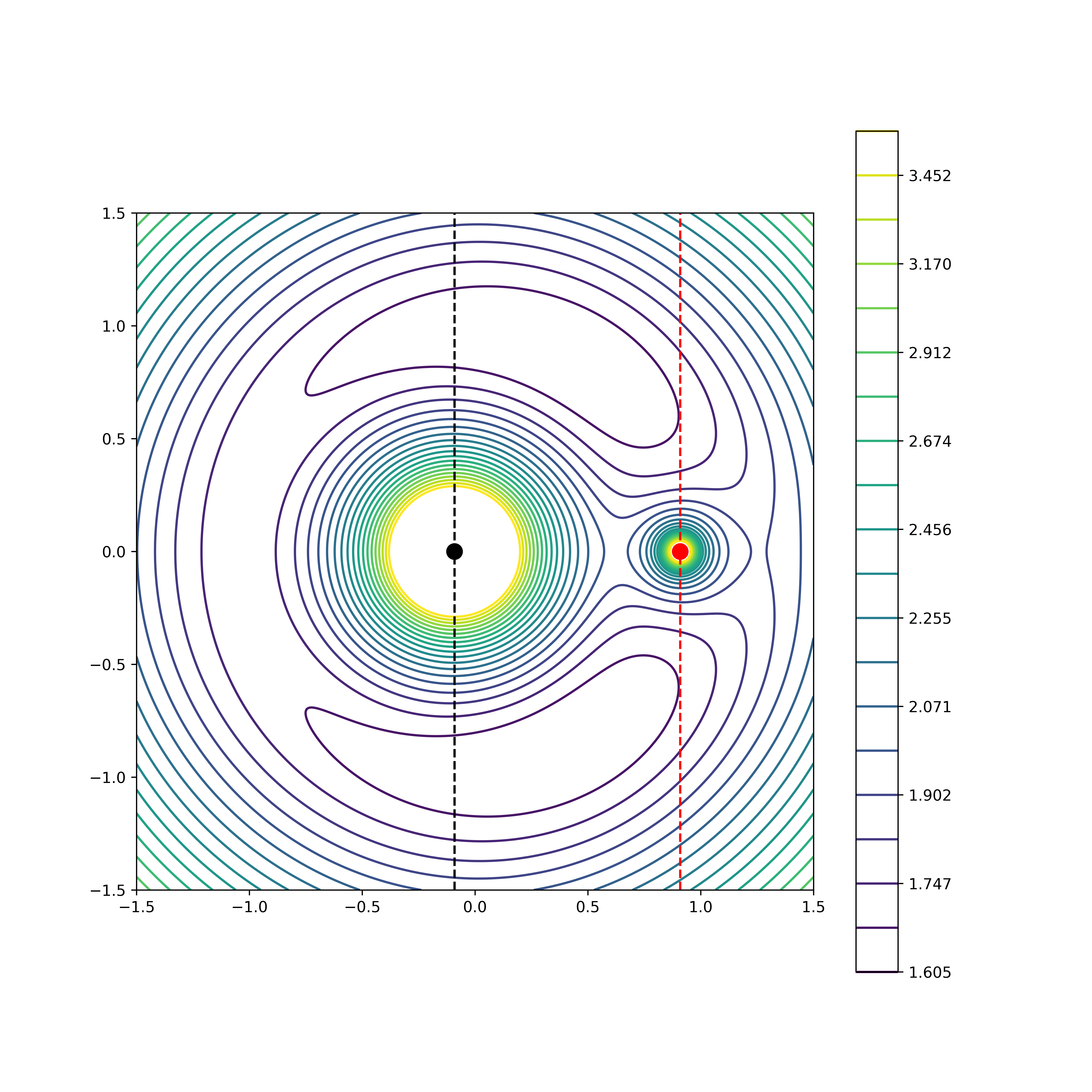Hence, $$C_j = -2 \mathcal{E} = n^2 (x^2 + y^2) + 2 \left( \frac{G m_1}{r_1} + \frac{G m_2}{r_2} \right) + \vec{v}^2 $$ Like energy, it is a constant of the motion. Additional insight can be gained through the examination of the terms in the constant. Except for the kinetic component, all these terms depend on the position of the test particle. Hence if we take \( \vec{v} = 0 \). We can plot the contours of this constant in space. If we plot these contours we obtain a figure like the one below.

A few things are worth noting. First, and most strikingly, the constant overall grows in near circles far from the planes. This is due to the centrifugal term, which grows quadratically with distance from the origin, while the gravitational terms shrink with distance. Second is that the constant is maximized at three locations, near \(m_1\), near \(m_2 \), and far from both masses. There are equilibria at a total of five points. Three on the x-axis (to the left and right of either body and between them) and two off-axis. These are the Lagrange points. In general, the points on the axis are always meta-stable, whereas the points off the axes are stable equilibria if the mass ratio \( \frac{m_1}{m_2} > \approx 25 \). It's also instructive to see what happens if we integrate the trajectory of our test particle for a few different initial conditions. In each case, we'll show the view both in the rotating frame and in the inertial frame, for comparison. We'll also show a black contour corresponding to the initial Jacobi constant of the particle. In our first case, we start the test particle close to \(m_1\) with only a small velocity. We see that the particle orbits \(m_1\) and never interacts with the second mass \( m_2\). Interstingly the trajectory in the rotating frame is bounded by our initial Jacobi constant. This is not surprising, since we assumed \( \vec{v} = 0 \) when we plotted the countors. Hence, when our particle reaches these contours, its velocity drops to zero, and it falls back towards the planet. These zero-velocity contours, then, act as impassable walls, through which the particle cannot penetrate. Evidently, for a particle with this Jacobi constant, there are only three 'types' of motion it can have. Either it orbits the primary mass and never visits the secondary, it orbits the secondary and never visits the primary, or it orbits both masses at a distance, never approaching either of them.

If we start the particle in the same position, but raise its velocity a bit, the zero velocity contours change, and a neck opens up between the primary and secondary regimes. While the trajectory is still confined to an inner domain between the bodies, it can now make close approaches to both and bounces between the two over time.

If we increase the velocity of the particle even further, the inner and outer regimes connect and the particle can leave the two-body system, though it can only do so by passing close to the outer mass. In the inertial frame, it's clear why this is. The particle must get an extra 'boost' from the orbiting mass in order to increase its velocity enough to escape.

It's worth noting the same is true from an outside perspective. If instead I change the situation and start the test particle external to the binary it will bounce along the zero velocity surface. It can only interact with the inner objects if its Jacobi constant is sufficiently small. In such a case, where the constant is just small enough to allow interaction, it must pass near the secondary to do so. If this is not true, and the Jacobi constant is a bit larger, then the test particle would be prevented from ever interacting with either inner body.